次浏览

一.Put forward Questions

1.1 Background

Data: https://datahack.analyticsvidhya.com/contest/practice-problem-loan-prediction-iii/

Tutorial: https://www.analyticsvidhya.com/blog/2016/01/complete-tutorial-learn-data-science-python-scratch-2/

1.2 Problem Statement

1.2.1 About Company

Dream Housing Finance company deals in all home loans. They have presence across all urban, semi urban and rural areas. Customer first apply for home loan after that company validates the customer eligibility for loan.

1.2.2 Problem

Company wants to automate the loan eligibility process (real time) based on customer detail provided while filling online application form. These details are Gender, Marital Status, Education, Number of Dependents, Income, Loan Amount, Credit History and others. To automate this process, they have given a problem to identify the customers segments, those are eligible for loan amount so that they can specifically target these customers. Here they have provided a partial data set.

1.3 Data

Variable | Description

Loan_ID	Unique Loan ID
Gender	Male/Female
Married	Applicant married(Y/N)
Dependents	Number of dependents
Education	Applicant Education (Graduate/ Under Graduate)
Self_Enployed	Self employed (Y/N)
ApplicantIncome	Applicant income
CoapplicantIncome	Coapplicant income
LoanAmount	Loan amount in thousands
Loan_Amount_Term	Term of loan in months
Credit_History	credit history meets guidelines
Property_Area	Urban/ Semi Urban/ Rural
Loan_Status	Loan approved (Y/N)

Note:

Evaluation Metric is accuracy i.e. percentage of loan approval you correctly predict.
You are expected to upload the solution in the format of “sample_submission.csv”

二. Solve Problem

2.1 Environment :

Ubuntu18.04 , Python3 , Numpy , Matplotlib , Pandas ,Sklearn

2.2 Exploratory analysis in Python using Pandas

2.2.1 Importing libraries and the data set and Quick Data Exploration:

	import numpy as np
	import pandas as pd
	import matplotlib.pyplot as plt
	df = pd.read_csv("train.csv")#Reading the dataset in a dataframe using Pandas
	print(df.head(10))
	print(df.describe())

This should print 10 rows. Alternately, you can also look at more rows by printing the dataset.
Next, you can look at summary of numerical fields by using describe() function.
Here are a few inferences:

LoanAmount has 614-592=22 missing values.
Loan_Amount_Term has 614-600=14 missing values.
Credit_History has 614-564=50 missing values.
The ApplicantIncome distribution seems to be in line with expectation. Same with CoapplicantIncome.

For the non-numerical values (e.g. Property_Area, Credit_History etc.), we can look at frequency distribution to understand whether they make sense or not. The frequency table can be printed by following command.Similarly, we can look at unique values of port of credit history.

	print(df['Property_Area'].value_counts())
	print(df['Credit_History'].value_counts())

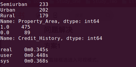We can also look that about 84% applicants have a credit_history.The mean of Credit_History field is 0.84 (475/564) (Remember, Credit_History has value 1 for those who have a credit history and 0 otherwise)

2.2.2 Distribution analysis

Now that we are familiar with basic data characteristics, let us study distribution of various variables. Let us start with numeric variables – namely ApplicantIncome and LoanAmount.

Lets start by plotting the histogram of ApplicantIncome using the following commands:

	print(df['ApplicantIncome'].hist(bins=50))
	pli.show()

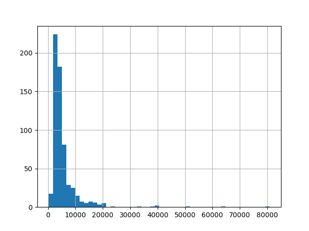Here we observe that there are few extreme values.This is also the reason why 50 bins are required to depict the distribution clearly.

Next, we look at box plot t ounderstand the distributions.Box plot for fare can be plotted by :

	print(df.boxplot(column='ApplicantIncome'))
	plt.show()

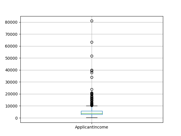This confirms the presence of a lot of outliers/extreme values. This can be attributed to the income disparity in the society. Part of this can be driven by the fact that we are looking at people with different education levels. Let us segregate them by Education:

	df.boxplot(column = 'ApplicantIncome',by ='Education')
	plt.show()

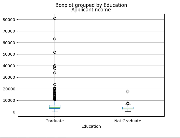We can see that there is no substantial different between the mean income of graduate and non-graduates. But there are a higher number of graduates with very high incomes, which are appearing to be the outliers.

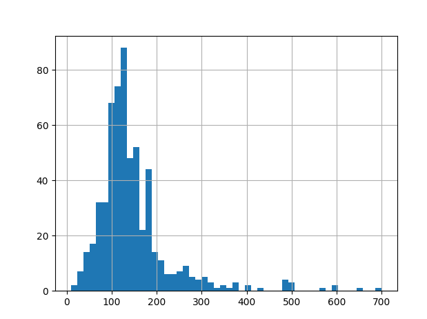
Now, Let’s look at the histogram and boxplot of LoanAmount using the following command:

	df['LoanAmount'].hist(bins=50)
	plt.show()

	df.boxplot(column='LoanAmount')
	plt.show()

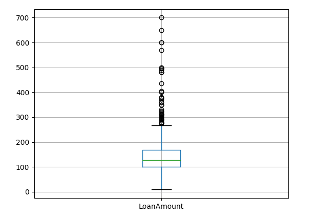Again, there are some extreme values.
Clearly, both ApplicantIncome and LoanAmount require some amount of data munging. LoanAmount has missing and well as extreme values values, while ApplicantIncome has a few extreme values, which demand deeper understanding. We will take this up in coming sections.

2.2.3 Categorical variable analysis

Now that we understand distributions for ApplicantIncome and LoanIncome, let us understand categorical variables in more details.

Loan Prediction Practice Problem

Using Python For Data Prediction